Group-level DE SNP Analsyis

Group-level SNP Analysis

Group level differential expression analysis requires a SNP database to be built (please see previous tutorials). This guide will walk you through the process of analyzing SNPs at the group level using the variantCell package.

Exploring SNP Metadata

To view the SNP metadata within your project, you can use the following command:

\dontrun{
  # Initialize a variantCell project
  project <- variantCell$new()
  
  # In practice, you would add samples and build the database first
  # project$addSampleData(...)
  # project$buildSNPDatabase()
  # project$setProjectIdentity("cell_type")

}

# View SNP metadata
View(project$snp_database$cell_metadata)

Creating Custom Metadata Variables

You can create new metadata variables to help with grouping or visualization:

# Create a combined patient and donor type variable
project$snp_database$cell_metadata$patient_donor <- paste0(
  project$snp_database$cell_metadata$patient, 
  '_', 
  project$snp_database$cell_metadata$donor_type
)

Aggregating SNP Counts by Group

Prior to analyzing SNP expression differences between groups, we need to aggregate the individual cell SNP counts into group-level summaries.

aggregateByGroup Function

# Function signature and parameters
project$aggregateByGroup(
  group_by,                # Column name in metadata to use for grouping cells
  donor_type = NULL,       # Specific donor type to analyze (e.g., "Donor" or "Recipient")
  min_cells_per_group = 3, # Minimum cells required per group
  use_normalized = TRUE    # Whether to use normalized counts
)

Example: Aggregating by Disease Status for Donor Cells

# Aggregate SNP counts by ACR status, using only donor cells
collapsed <- project$aggregateByGroup(
  group_by = "snpGrade",     # Group by ACR status
  use_normalized = TRUE,     # Use normalized counts
  donor_type = 'Donor'       # Restrict to donor cells only
)

When executed, you should see output similar to:

Filtering for donor type: Donor
Total cells before filter: 56676
Cells passing filter: 22096
NA values in donor_type: 1003

Collapsed data by snpGrade:
 - Total cells: 22096
 - Total groups: 2
 - Included groups: 2
 - Filtered groups: 0
 - Using normalized counts: TRUE

Group details:
   group n_cells mean_depth filter_status
1    ACR   12598   3981.279      included
2 No_ACR    9498   7392.881      included

Finding Differentially Expressed SNPs Between Groups

After aggregating our data, we can identify SNPs that are differentially present between groups. The findSNPsByGroup function compares alternative allele frequencies between groups to find variants that are specifically present in one group but not the other.

findSNPsByGroup Function

# Function signature and parameters
project$findSNPsByGroup(
  ident.1,                 # Primary group identity to analyze
  ident.2 = NULL,          # Secondary group identity to compare against (NULL = all others)
  aggregated_data,         # Output from aggregateByGroup function
  min_depth = 10,          # Minimum read depth required for a group
  min_alt_frac = 0.2,      # Minimum alt allele fraction in primary group
  max_alt_frac_other = 0.1, # Maximum alt fraction allowed in other group
  return_all = TRUE        # Whether to return all results or only significant ones
)

Example: Finding SNPs Between ACR and No_ACR Groups

# Find SNPs present in ACR patients but absent in No_ACR patients
de_results <- project$findSNPsByGroup(
  ident.1 = "ACR",             # Primary group to analyze
  ident.2 = 'No_ACR',          # Comparison group
  aggregated_data = collapsed, # Aggregated data from previous step
  min_alt_frac = 0.05,         # SNP must have at least 5% alt frequency in ACR
  max_alt_frac_other = 0.01    # SNP must have no more than 1% alt frequency in No_ACR
)

Examining the Results

After running the analysis, you can examine the results:

# View summary of the analysis
print(de_results$summary)

# Look at the top SNPs by presence score
head(de_results$results[order(-de_results$results$presence_score), ], 10)

# How many SNPs are present in each group?
table(de_results$results$presence)

# Save results to a CSV file
write.csv(de_results$results, 'SNP_ACR_NoACR_Donor.csv', row.names = FALSE)

Visualizing SNPs in Genes of Interest

You can visualize SNPs within specific genes using the plotSNPs function.

plotSNPs Function

# Function signature and parameters
project$plotSNPs(
  gene,                      # Gene symbol to visualize
  group.by = NULL,           # Primary grouping variable from metadata
  split.by = NULL,           # Secondary grouping variable for within-group comparisons
  idents = NULL,             # Specific identity values to include
  min_depth = 10,            # Minimum read depth required for a SNP
  min_cells = 3,             # Minimum cells per group required
  min_alt_frac = 0.2,        # Minimum alternative allele fraction
  flank_size = 5000,         # Size of flanking regions (bp) around gene
  plot_density = TRUE,       # Whether to include density plots
  data_out = FALSE,          # Return data frame instead of plots
  use_normalized = FALSE,    # Use normalized read depth values
  color_scheme = c("low" = "blue", "high" = "red"), # Colors for gradient
  point_size_range = c(2, 8) # Range of point sizes for depth
)

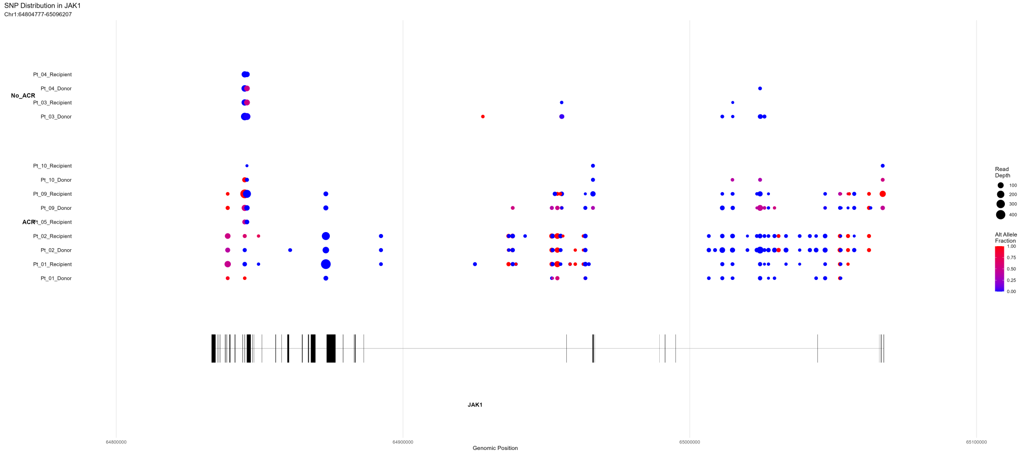
Example: Visualizing JAK1 SNPs by ACR Status and Patient-Donor

# Plot SNPs in JAK1 gene without minimum alt fraction threshold
project$plotSNPs(
  'JAK1',
  group.by = 'snpGrade',       # Group by ACR status
  split.by = 'patient_donor',  # Split by patient and donor type
  min_alt_frac = 0,            # Show all SNPs regardless of alt fraction
  plot_density = FALSE         # Don't show density plots
)

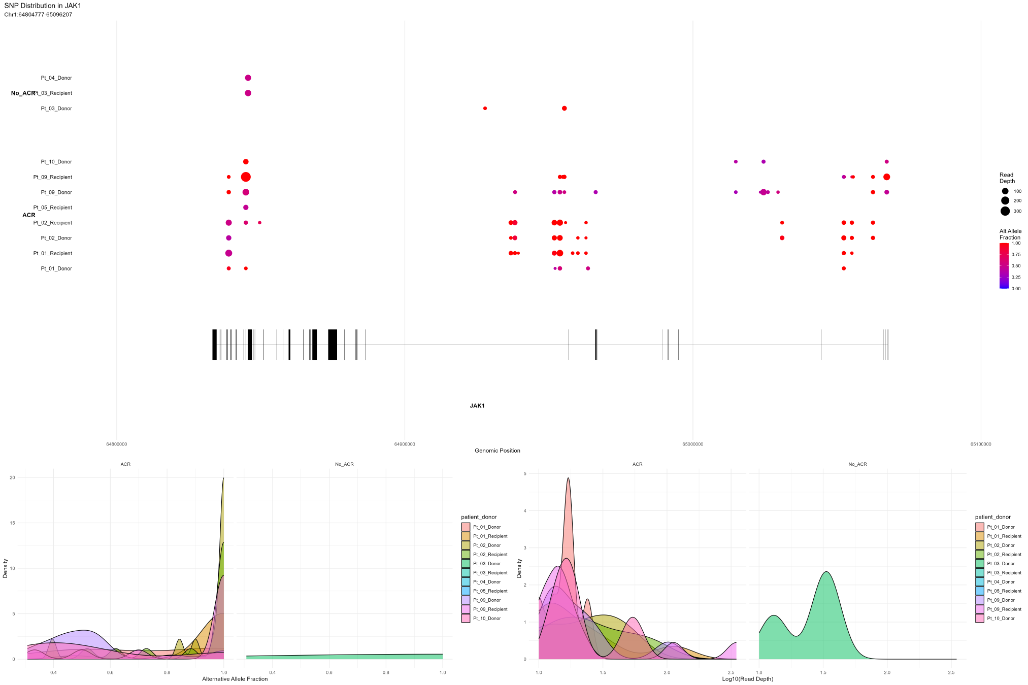
Example: Visualizing With Filtered SNPs and Density Plots

# Plot JAK1 SNPs with minimum alt fraction and density plots
project$plotSNPs(
  'JAK1',
  group.by = 'snpGrade',
  split.by = 'patient_donor',
  min_alt_frac = 0.2,         # Only show SNPs with alt fraction ≥ 0.2
  plot_density = TRUE         # Include density plots
)

# Get SNP data for JAK1 as a data frame
jak1_data <- project$plotSNPs(
  'JAK1',
  group.by = 'snpGrade',
  split.by = 'patient_donor',
  min_alt_frac = 0,
  data_out = TRUE             # Return data frame instead of plot
)

# Save to CSV for external analysis
write.csv(jak1_data, "JAK1_SNPs.csv", row.names = FALSE)

Andrew Potter

2025-05-12